

Read the video transcript
Aharon Ben-Tal was an important reference during my PhD in operations research. His John von Neumann Theory Prize is a good occasion to explain an idea that matters far beyond academia: robust optimization.
Imagine a factory planning next week's production with one hundred machine-hours. Once its product mix is released, quantities can be cut, but no quantity can be increased that week. These are hypothetical numbers for teaching.
Product A contributes ninety dollars per batch and takes two machine-hours. Product B contributes fifty dollars and nominally takes one hour. The factory can sell at most forty batches of A and sixty of B.
At those times, the optimal plan makes twenty batches of A and sixty of B. It uses exactly one hundred hours and generates forty-eight hundred dollars in contribution margin. Every available hour is committed.
Now B takes one point two five hours per batch. The planned mix needs one hundred fifteen hours, but the machine stops after one hundred. Some production must be left unfinished. What contribution margin can the factory actually deliver?
Give the nominal plan the best possible repair. Finish its twenty batches of A and forty-eight of B. That uses all one hundred hours and realizes forty-two hundred dollars. Twelve planned batches of B are deferred. The shortfall is six hundred dollars of contribution margin, even before adding any late-delivery penalties.
Robust optimization considers the uncertainty before choosing the mix. Here, B can take between zero point seven five and one point two five hours. We require the plan to fit throughout that interval, including favorable and unfavorable conditions.
The robust plan commits to forty batches of A and sixteen of B. At the slow processing time, it completes every planned batch in exactly one hundred hours and realizes forty-four hundred dollars in contribution margin.
Compare execution with execution: forty-two hundred dollars from the best cut of the nominal plan, versus forty-four hundred from the robust plan. The robust mix delivers two hundred dollars more in the same slow week, with none of its own batches deferred.
Now let B take just zero point seven five hours. The nominal plan completes everything in eighty-five hours and realizes forty-eight hundred dollars. The robust plan uses ninety-two hours and realizes forty-four hundred. It gives up four hundred dollars of upside. The spare hours cannot create extra batches because the mix is already committed.
The robust plan gives up four hundred dollars when conditions are favorable or nominal. It delivers two hundred more when processing slows down. Those are the opportunity costs we need to compare before deciding what protection is worth.
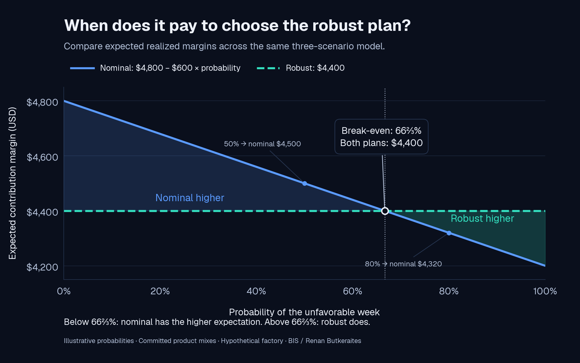
To calculate expected margin, weight each realized outcome by its probability. With a fifty percent chance of the slow week, the nominal plan averages forty-five hundred dollars, above the robust forty-four hundred. At eighty percent, it averages forty-three hundred twenty, below the robust plan. Robust planning wins in expectation above a two-thirds slow-week probability in this example. These probabilities are illustrative.
The robust guarantee covers the chosen interval, without requiring probabilities. A time outside that interval can still break the plan. Probabilities are additional assumptions for comparing expected economic outcomes.
Ben-Tal and his collaborators helped build the foundations for decisions like these. His work was an important part of my formation as a researcher. Compare what your plans can actually deliver when conditions change. The full example is on the BIS blog.
Aharon Ben-Tal was an important reference during my PhD in operations research. Reading that INFORMS had awarded him the 2026 John von Neumann Theory Prize brought me back to a question at the center of optimization under uncertainty: what happens to a good decision when the data change? The award was announced on October 19 and recognizes his sustained contributions, particularly his pioneering work on robust optimization.1
A production schedule can be mathematically optimal and still fail on the shop floor. The solver may be correct. The processing times it was given may be too precise for the operation they describe. Robust optimization brings that uncertainty into the decision itself.
One factory, two products, 100 machine-hours
Consider a hypothetical factory choosing next week's production mix. All the numbers below are invented for teaching and calculated exactly; they are not results from a client engagement. Quantities are whole production batches. Contribution margin is revenue minus variable costs, before fixed costs.
| Product | Contribution per batch | Machine-hours per batch | Maximum weekly sales |
|---|---|---|---|
| A | $90 | 2 hours, treated as fixed | 40 batches |
| B | $50 | 1 hour nominal; range 0.75–1.25 hours | 60 batches |
The factory has 100 machine-hours available. There is no overtime or outsourcing in this model, and margins, sales limits, and A's processing time are held fixed. B's time is uncertain because material quality or operating conditions can speed up or slow processing. For the example, we assume its weekly processing time per batch lies anywhere between 0.75 and 1.25 hours, around a nominal one hour. Once the weekly mix is released and product-specific inputs are reserved, quantities can be reduced, but no product's quantity can be increased during that week. Both approaches face this same commitment rule.
The nominal optimum uses every hour
Using the nominal times, B earns $50 per machine-hour while A earns $45. The best plan makes 60 batches of B and 20 of A. It uses exactly 100 hours and produces $4,800 of planned contribution margin: 60 × $50 + 20 × $90.
Now let B take 1.25 hours per batch. The same plan requires 60 × 1.25 + 20 × 2 = 115 hours. The machine stops after 100. The factory cannot realize the promised $4,800 within that capacity, so some planned production must be left unfinished.
What can the nominal plan actually deliver?
Give the nominal plan the best possible repair after the slowdown is known. Choose the most profitable subset of its released batches: maximize 90A + 50B, subject to 2A + 1.25B ≤ 100, A ≤ 20, B ≤ 60, and whole, nonnegative batches. This allows intelligent reprioritization instead of assuming an arbitrary production sequence or proportional cut.
At the slow time, A contributes $45 per machine-hour and B contributes $40. Complete all 20 planned batches of A, using 40 hours. The remaining 60 hours complete 48 batches of B. The best executable cut therefore realizes $4,200: 20 × $90 + 48 × $50. It uses all 100 hours, but 12 of the 60 planned B batches remain unproduced this week. These are deferred batches, not 15 idle machine-hours.
The shortfall against the original plan is $600 of contribution margin, or 12.5%. Realized margin here counts only completed, sold batches at the stated per-batch contributions. No late-delivery penalty, spoilage charge, inventory carrying cost, or extra cost for reserved inputs is added. This is an illustrative execution model, not a measured client loss.
Choose the mix while accounting for the uncertainty
In a static robust model, we choose the batches before the processing time is known and require the capacity constraint to hold for every time in the chosen uncertainty set. This example uses the interval tB ∈ [0.75, 1.25]. The guarantee is conditional on that interval and on the rest of our model.2
Because production is nonnegative, the largest machine load occurs at tB = 1.25. The robust capacity constraint is therefore 2A + 1.25B ≤ 100, together with whole-batch limits 0 ≤ A ≤ 40 and 0 ≤ B ≤ 60. We still maximize the same contribution margin, 90A + 50B.
The best robust plan makes 40 batches of A and 16 of B. Its contribution margin is $4,400. It uses 92 hours in the favorable case, 96 at the nominal processing time, and exactly 100 at the slow end of the interval. Every intermediate processing time also fits. Allowing favorable processing times does not change this robust solution, because the upper endpoint still determines the largest machine load.
| Measure | Nominal plan | Robust plan |
|---|---|---|
| Batches of A / B | 20 / 60 | 40 / 16 |
| Planned contribution margin | $4,800 | $4,400 |
| Hours when B takes 0.75 hours | 85 | 92 |
| Hours when B takes 1 hour | 100 | 96 |
| Hours when B takes 1.25 hours | 115 | 100 |
Compare execution with execution
In the same slow week, the robust plan completes its 40 batches of A and 16 of B within 100 hours and realizes $4,400. The best repair of the nominal plan realizes $4,200 in those same 100 hours. Robust planning delivers $200 more contribution margin, about 4.8% above the repaired nominal plan, with none of its own planned batches deferred.
| Slow-week outcome | Best repair of nominal plan | Robust plan |
|---|---|---|
| Completed batches A / B | 20 / 48 | 40 / 16 |
| Unproduced from own plan | 12 batches of B | 0 batches |
| Machine-hours actually used | 100 | 100 |
| Realized contribution margin | $4,200 | $4,400 |
| Shortfall against own planned margin | $600 | $0 |
What if the best case happens?
Now let B take only 0.75 hours: a favorable realization, 25% less processing time than the nominal assumption. The nominal plan completes all 20 A and 60 B batches in 85 hours and realizes $4,800. The robust plan completes its 40 A and 16 B batches in 92 hours and realizes $4,400. The nominal plan wins by $400 in this favorable case, just as it does at the nominal processing time.
The faster machine does not automatically create extra sales in this example. Both mixes are already released, and the same no-increase rule applies. The nominal plan leaves 15 hours unused; the robust plan leaves eight. Those hours are available capacity, distinct from the 12 planned batches left unfinished in the slow nominal execution. A factory that can add batches or switch products after the reveal needs an execution model that includes those options.
| Scenario | B time per batch | Nominal realized margin | Robust realized margin | Best margin if known before release |
|---|---|---|---|---|
| Favorable | 0.75 h | $4,800 | $4,400 | $5,430 |
| Nominal | 1 h | $4,800 | $4,400 | $4,800 |
| Unfavorable | 1.25 h | $4,200 | $4,400 | $4,400 |
If the favorable processing time were known before release, the best integer mix would be 27 A and 60 B, using 99 hours and generating $5,430. Relative to that full-information benchmark, the nominal plan leaves $630 of achievable margin on the table and the robust plan leaves $1,030. This benchmark prices the missed upside; it is not a plan that can be chosen after observing the future under our commitment rule. In the slow case, the robust mix already matches the full-information optimum, while the nominal execution falls $200 short.
Protection has a price you can inspect
The opportunity cost depends on which conditions occur. At the nominal processing time, the nominal plan realizes $4,800 and the robust plan realizes $4,400: protection costs $400, or 8.3% of nominal margin. In the slow week, the nominal plan's execution shortfall is $600. The robust plan's $400 initial concession is then more than offset, leaving a $200 realized advantage. The broader trade-off between nominal performance and protection is a central topic in the robust optimization literature.3
| Realized time for B | Nominal plan, after any cuts | Robust plan | Robust minus nominal |
|---|---|---|---|
| 0.75 hours · favorable | $4,800 | $4,400 | −$400 |
| 1 hour | $4,800 | $4,400 | −$400 |
| 1.25 hours | $4,200 | $4,400 | +$200 |
Robust planning makes economic sense here when the value of avoiding execution shortfalls justifies the nominal margin given up. It does not promise a higher margin in every scenario. If the mix could be changed freely after observing the slowdown, the nominal planner could also move to 40 batches of A and 16 of B. The advantage in this comparison comes from anticipating uncertainty before commitments restrict what can be changed.
For an expected-value illustration, assign probabilities pF, pN, and pU to the favorable, nominal, and unfavorable scenarios, summing to one. The nominal plan's expected realized margin is 4,800pF + 4,800pN + 4,200pU = 4,800 − 600pU. The robust plan's is 4,400 in every displayed scenario, so its expectation is also 4,400. These are assumed discrete scenarios for the economic calculation; they do not assign probabilities to the entire continuous uncertainty interval.
| Probabilities: favorable / nominal / unfavorable | Nominal expected margin | Robust expected margin | Higher expected margin |
|---|---|---|---|
| 25% / 25% / 50% | $4,500 | $4,400 | Nominal by $100 |
| 10% / 10% / 80% | $4,320 | $4,400 | Robust by $80 |
Calculate the expected contribution margin
These are illustrative probabilities, not measurements. Favorable and nominal weeks split the remaining probability equally. Their realized margins are the same under the committed production mixes.
Favorable: 25% · Nominal: 25% · Unfavorable: 50%
Expected contribution margin · USD
Nominal is higher by $100 in expectation under these probabilities.
Nominal expectation = $4,800 − $600 × probability of the unfavorable week. Break-even: 66⅔%. These probabilities weight only the three displayed scenarios. They are separate from the robust feasibility guarantee over the entire 0.75–1.25 hour interval.
In this three-scenario illustration, robust planning has the higher expected margin when the unfavorable scenario's probability exceeds two-thirds. Below that threshold, the nominal plan has the higher expectation; the robust plan still has the higher minimum realized margin, $4,400 versus $4,200. Selecting the highest expected value and protecting a minimum are different objectives. Real operations may have intermediate outcomes, penalties, and more expensive recourse; those belong in the economic comparison rather than being assumed away or invented to favor a result.
The change is more deliberate than cutting every quantity by a fixed safety factor. At the slow processing time, A earns $45 per hour and B earns $40. The optimizer shifts production toward A, up to its sales limit, and uses the remaining capacity for B. It chooses both the amount of production and its composition.
The uncertainty set is an operational assumption
If B takes 1.4 hours, the robust plan needs 102.4 hours and exceeds capacity. That outcome is outside our chosen interval. Calling a plan robust never means it survives every possible disruption. It means its constraints hold over a specified set of parameter values.
A real project must justify that set using process measurements, engineering knowledge, and the consequences of failure. Making it wider can buy more protection and reduce planned performance. With many uncertain inputs, their dependence and which combinations are plausible matter too. Probability guarantees require additional assumptions or statistical calibration; an interval alone does not give a 95% service level.
Other models answer other operational questions. A stochastic model can use probabilities and optimize expected performance; a chance constraint can specify a probability of meeting a requirement. Adjustable robust optimization lets some decisions respond after information arrives. The right choice depends on what is known and when the factory can act.4
Why Ben-Tal's work matters to me
Ben-Tal, together with collaborators including Arkadi Nemirovski and Laurent El Ghaoui, helped establish mathematical tools for turning uncertainty sets into optimization problems that can be solved efficiently for important problem classes. The geometry of the set affects the resulting model. Our one-interval example is a deliberately simple illustration, not a reproduction of one of his specific algorithms.2
His work was an important reference during my doctorate. This recognition is an opportunity to acknowledge that influence and make the underlying question concrete: what uncertainty are we willing to plan for, what should remain feasible, and how much planned performance are we willing to exchange for that protection? In a factory, those questions show up as product mixes, machine-hours, and promises made to customers.
How the example was checked
All 2,501 integer production mixes were enumerated for each planning model, and all 1,281 possible subsets of the nominal mix were checked for execution. Optimality also has a short independent check. For the nominal planning model, 90A + 50B = 45(2A + B) + 5B ≤ 45 × 100 + 5 × 60 = 4,800. For the robust model, 90A + 50B = 40(2A + 1.25B) + 10A ≤ 40 × 100 + 10 × 40 = 4,400. For the nominal plan's best slow-week repair, the same identity with A ≤ 20 gives an upper bound of 40 × 100 + 10 × 20 = 4,200. All three plans attain their respective bounds. Monotonicity in B's processing time establishes robust feasibility over the full interval, without relying on simulation.